SNOSWAB
Snow, Soil Water and Water Balance Model
Online Tool
-
1. About SNOSWAB
SNOSWAB (Snow, Soil Water and Water Balance Model) is an online tool for obtaining daily estimates of snow related processes (e.g., snowfall, snowmelt, snow layer thickness), soil water content and a series of soil water budget components (e.g., infiltration, drainage, surface runoff) based on user provided daily meteorological (i.e., mean air temperature, total precipitation, rainfall), evapotranspiration and calibration data. SNOSWAB has been developed through a collaborative research effort between Canadian Rivers Institute (CRI), University of New Brunswick (UNB), Agriculture and Agri-Food Canada (AAFC) and Environment and Climate Change Canada (ECCC). SNOSWAB is a result of a larger research effort aimed at evaluating the effects of agricultural production systems on groundwater and surface water quantity and quality. SNOSWAB is part of the Hydrology Tool Set (HTS; https://www.hydrotools.tech), a suite of tools that can be used for advancing the understanding of various local and watershed scale hydrological processes. HTS also includes SepHydro (daily baseflow / hydrograph separation; 11 methods), ETCalc (daily potential, reference and actual evapotranspiration estimation; 8 methods), SWIB (daily estimation of soil water stress, crop water deficit, irrigation requirement and its impact on aquifer storage, water budget components), GWRech (daily estimation of groundwater recharge and groundwater discharge), TotPrePart (partitioning of daily total precipitation into snowfall and rainfall) and FLEX-WQI (estimation of water quality state via water quality indexes).
If you used SNOSWAB, please include the following citation(s) in your publication(s):
Danielescu S (2024) Development and Application of the Snow, Soil Water and Water Balance Model (SNOSWAB), an Online Model for Daily Estimation of Snowpack Processes, Soil Water Content and Soil Water Balance. Water 16: 1503.
DOI: https://doi.org/10.3390/w16111503.Danielescu S, MacQuarrie KTB, Nyiraneza J, Zebarth B, Sharifi-Mood N, Grimmett M, Main T, Levesque M (2024) Development and Validation of a Crop and Nitrate Leaching Model for Potato Cropping Systems in a Temperate–Humid Region. Water 16: 475.
DOI: https://doi.org/10.3390/w16030475. -
2. Background
The water balance is an important hydrological tool that allows for quantification of the flow of water in and out of a system as well as of the amount of water available in the system. Understanding of the water balance provides the basis for advancing our understanding relative to hydrological cycle, ecosystem health or agroecosystem productivity and can be an important tool for water-resource management and environmental planning. Examples of application of water balance include evaluation of the impacts of climate variability and severe weather (e.g., droughts) on water availability; impact of human activities on water resources; the impact of water stress (water deficit and excess) on natural vegetation and agricultural crops; movement of water and solutes (e.g., contaminants) through soil; irrigation requirements for agricultural production, etc.
SNOSWAB (Snow, Soil Water and Water Balance tool) integrates several components that allow for estimation of daily dynamics and magnitude of various water balance components. SNOSWAB provides routines for estimation of snow related processes, soil water content and soil water budget terms. SNOSWAB also allows for simulation of water additions (e.g., irrigation), and water subtractions (e.g. passive drainage via tile drains or dewatering via pumping) to and from the soil layer. SNOSWAB can be applied to any location for which input data is available and can be used for evaluating various scenarios relevant for the above processes. The model includes extensive calibration routines when user-provided calibration data is available. The web-based model provides various data visualization, analysis and output options through a streamlined process and a user-friendly interface.
SNOSWAB integrates four modules: 1) HOME; 2) INPUT DATA; 3) SNOW; and 4) WATER BALANCE.
The HOME module contains information regarding the context of model development, a presentation of the various concepts used and the user guide.
The INPUT DATA module provides an interface for uploading user time series data or for loading the provided test data to the model. The Test Data set allows users to test the various routines and familiarize themselves with the model.
The SNOW module allows for estimation of a series of snow related processes (e.g., snowfall, snowmelt, snow layer thickness) and produces the amount of water available (i.e., water available for infiltration and surface runoff) for calculations carried out in the next module.
The WATER BALANCE module allows for daily estimation of soil water content and of a series of water budget components (e.g., infiltration, drainage, surface runoff). In addition, this module allows for visualization of the water budget and model error using a dynamic water budget diagram and its associated (simplified) table.
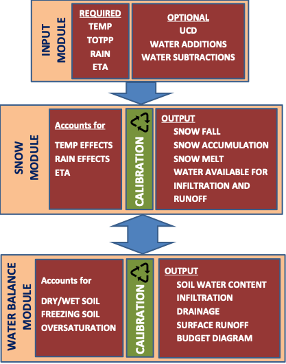
Fig 1. Simplified workflow diagram for SNOSWAB model
TEMP - daily mean air temperature; TOTPP - daily total precipitation; RAIN - daily rain; ETA - daily actual (or crop) evapotranspiration; UCD - user calibration data
-
3. Methodology
Details regarding data management as well as the methodology used for each SNOSWAB module are included below.
3.1. Input Data File
The Input Data file consists of a collection of daily time series including both required and optional data. SNOSWAB allows uploading of files with maximum 7500 rows (~20 years of daily data). It is recommended to split the input data set in blocks of 20 years daily timeseries when the intent is to analyze longer time periods.
The REQUIRED INPUT TIME SERIES is a daily dataset required for conducting analyses using SNOSWAB. The required input time series data includes:
-
Air temperature (TEMP). This is a parameter used by the SNOW module. TEMP is required for calculation of a series of snow and drainage related processes. TEMP represents the daily mean air temperature and is typically available from in situ measurements or from other sources (e.g., weather stations, online databases, etc.). The units for TEMP are ° C;
-
Total precipitation (TOTPP). This is a parameter used by the SNOW module. TOTPP is required for calculation of a series of snow and infiltration related processes. TOTPP represents the daily total precipitation and includes all forms of precipitation (e.g., snow, rain, freezing rain, etc.). TOTPP is available from in situ measurements or from other sources (e.g., weather stations, online databases, etc.). The units for TOTPP are mm;
-
Rain (RAIN). This is a parameter used by the SNOW module. RAIN is required for calculation of a series of snow and infiltration related processes. RAIN represents the daily rainfall. RAIN is available from in situ measurements or from other sources (e.g., weather stations, online databases, etc.). In the absence of direct measurements, daily rainfall can be estimated using SNOWFALL BUDDY (Snowfall and Rainfall Estimation Tool), a tool included in the Hydrology Tool Set (HTS) and available at https://sbuddy.hydrotools.tech. SNOWFALL BUDDY allows for estimation of both snowfall and rainfall amounts based on total precipitation and air temperature. The units for RAIN are mm;
-
Evapotranspiration (ETA). This is a parameter used by the SNOW and WATER BALANCE modules. ETA is required for calculation of a series of snow and infiltration related processes. ETA represents the daily actual (or crop) evapotranspiration. ETA is generally not readily available from weather stations; however it can be obtained from in situ measurements or from other sources (e.g., weather stations, online databases, etc.). If not directly available to the user, evapotranspiration can be calculated on a daily basis using ETCalc, a tool included in the Hydrology Tool Set (HTS) and available at https://etcalc.hydrotools.tech. ETCalc allows for estimation of daily potential evapotranspiration, reference evapotranspiration and actual evapotranspiration. The units for ETA are mm;
The OPTIONAL INPUT TIME SERIES includes water additions and subtractions as well as User Calibration Data (UCD).
Water additions and subtractions datasets include timeseries that can be used as input data for SNOSWAB calculations.
Water additions represent the amount of water added to the system from sources other than precipitation (e.g. irrigation, flooding, etc.). Water additions are applied to the top of the soil and are used in the calculation of the amount of water available for infiltration or surface runoff. During the SNOSWAB simulation setup the user is provided with the option of using water additions from the input file.
Water subtractions represent the amount of the water that is removed from the system either via diversions or dewatering.
Water subtractions via diversions represent the amount of water passively removed from the soil layer (e.g. via tile drainage). During SNOSWAB calculations, water subtractions via diversions is removed from drainage, and is limited by the amount of water available for drainage. In addition to being able to use the water subtractions via diversions from the input file, SNOSWAB can also simulate water subtractions via diversions as a fixed portion of the drainage. The simulated water subtractions via diversions are added to the amounts available in the input file if the user chooses to use both options during the SNOSWAB setup process.
Water subtractions via dewatering represent the amount of water actively removed from the soil layer (e.g. via pumping). During SNOSWAB calculations, water subtractions via dewatering is removed from the amount of the water stored in soil (i.e.; soil water content), and is subject to additional conditions controlling the availability of water for dewatering. In addition to being able to use the water subtractions via dewatering from the input file, SNOSWAB can also simulate water subtractions via dewatering by using the user-specified dewatering rate and the soil water content threshold for activating the simulated dewatering routine. The simulated water subtractions via dewatering are added to the amounts available in the input file if the user chooses to use both options during the SNOSWAB setup process.
UCDs are daily datasets used for calibrating SNOSWAB output. The user calibration data (UCD) is critical for guiding the calibration of the model. In the absence of the UCD data, the SNOSWAB model cannot be calibrated. The users can upload (up to) 5 columns of daily input datasets for model calibration. The format of the optional input time series is restricted to numerical values and the user is provided the option of pairing these time series with parameters calculated by SNOSWAB during the calibration process. UCD data sets are not restricted to certain parameters and can include daily time series for any parameter that the user intends to use for comparing with the output from SNOSWAB. Examples of calibration time series datasets include thickness of snow layer, soil water content, groundwater recharge, stream baseflow, surface runoff, etc.
The number of columns, data format and the units of the various weather parameters required for the input file are shown in the table below.
Columns DATE TEMP TOTPP RAIN ETA WADD WDIVinp DEWAinp UCD (max. 5 cols.) Units yyyy-mm-dd °C mm mm mm mm mm mm user choice Values eg. 2021-12-24 -90 to 60 0 to 1800 0 to 1800 0 to 100 >= 0 >= 0 >= 0 user choice
Notes:
-
Required data:
DATE - use yyyy-mm-dd format;
TEMP - daily mean air temperature;
TOTPP - daily total precipitation;
RAIN - daily rain;
ETA - daily actual (or crop) evapotranspiration; -
Optional data: (leave blank if no data is available)
WADD - daily water additions
WDIVinp - daily water subtractions via diversions
DEWAinp - daily water subtractions via dewatering
UCD - user calibration data (up to five columns) -
The model requires daily data
-
The user input data file has to be uploaded using a file with one column dedicated to calendar date, four columns dedicated to required input data (TEMP, TOTPP, RAIN, ETA), three columns dedicated to optional input data (WADD, WDIVinp, DEWAinp) and up to five columns dedicated to calibration data (UCD1 to UCD5)
-
Use the first row of the data set for column headings
-
SNOSWAB includes limited input data quality check routines and hence, the user must ensure that the input data set is suitable for analysis (e.g., check dataset for missing or erroneous values, etc.)
In addition to the input data timeseries, SNOSWAB requires a series of coefficients (see section 3.3.)
3.2. Time steps and averaging
SNOSWAB uses daily data for both input and output data. SNOSWAB includes a series of averaging options (i.e., monthly, seasonal [meteorological and growing season], yearly), which are explained in more detail below. SNOSWAB can also calculate all the output parameters using a "typical year daily" (i.e., daily multi-year averages for each day of the year available in the input and output files) for the cases when the analysis is carried out for a period longer than one year. The daily values for the typical year can also be averaged over monthly, seasonal [meteorological and growing season], and for the entire period covered by the datasets. The following time intervals are available in tables, graphs and export files for displaying SNOSWAB results:
-
Daily: this is the operating time step for SWIB;
-
Monthly;
-
Yearly;
-
Meteorological seasons, with the following distribution: Spring: March 1 - May 31st; Summer: June 1st - August 31st; Fall: September 1st - November 30th; Winter: December 1st - February 28th of the following year;
-
Growing season [GS] and outside of growing season [OGS], based on the starting and ending dates specified by the user. OGS spans between the first day after the end of the growing season and the day before the start of the following year’s growing season;
-
Typical year daily: one year of daily data based on the averages of the output data for each day in multiple years (i.e., 365 values) (e.g. for a 5-year daily data set, the value for Jan 1 will be the average for the values on Jan 1 in Year 1,2, 3, 4, and 5). This could be interpreted as the "representative daily year" or "average daily year";
-
Typical year monthly: one year of monthly averages (i.e., 12 values). The monthly averages are calculated using the typical year daily values;
-
Typical year meteorological season: meteorological season averages (i.e., four values). The meteorological season averages are calculated using the typical year daily values;
-
Typical year growing season: growing season (GS) and outside of growing season (OGS) averages (i.e., two values). The growing season averages are calculated using the typical year daily values;
-
Yearly: the average for all days in the typical year daily (i.e., one value).
3.3. Model Settings and Coefficients
-
Input Data Module
Start and end date for the growing season. Used for allowing SNOSWAB to calculate all the parameters for the growing season (GS) and outside of the growing season (OGS) in addition to other averaging periods. The start and end dates use mm-dd format (the year is ignored as the same dates are applied to all years available in the input data file).
-
Snow Module
The settings and coefficients used by the SNOW module are required both for running and calibrating the model. The settings and values of the coefficients can be set up manually using the collapsible menus available under the Analysis Tab or can be uploaded as a set using the “Import configuration file” button available in the same tab. The configuration file can be downloaded using the “Export Configuration File” button under the Analysis Tab (including either default settings and values of the coefficients if the first model run has not been completed or settings and values of the coefficients as set for the last available run of the model if the analysis has been completed at least once) or by using “Export Snow Configuration” in the “Export Snow Data” menu (available after one successful run of the module). The adjusted settings and values of the coefficients can be restored to default values by using the "Reset to Default" button available at the bottom of the page in the Analysis tab.
WATER ADDITIONS NAME LONG NAME DEFINITION VALUES WADD Water additions from input file (mm) The amount of water added to the soil from sources other than precipitation (e.g. irrigation, flooding, etc.). Water additions are applied to the top of the soil and are used in the calculation of the amount of water available for infiltration or surface runoff. Leave the box unchecked if water addition data is not available in the input file or if the intent is not to use it in calculations. n/a STARTING VALUES NAME LONG NAME DEFINITION VALUES SNWTinit Initial snow layer thickness (cm) Thickness of the snow layer on the first day of the analysis. This is converted into mm for subsequent calculations using 1/CFSmc. ≥ 0 SNWMinit Initial snowmelt (mm) Amount of snow melted on the first day of the analysis. ≥ 0 COEFFICIENTS NAME LONG NAME DEFINITION VALUES THRrs Air temperature threshold for rain to be accumulated as snow (° C) Precipitation falling as rain is treated as snow when air temperature is below this threshold. This results in the respective rain amount to be added to the snow layer instead of infiltrating and/or becoming surface runoff. -20 to 10 THRsm Air temperature threshold for initiating snowmelt (° C) Precipitation falling as snow is treated as rain when air temperature is above this threshold. In addition, melting of the snow occurs on days with air temperature above this threshold. -20 to 10 CFTsm Correction factor - snowmelt due to air temperature (mm) The amount of snow that is melted for each degree of air temperature above THRsm. ≥ 0 CFRsm Correction factor - snowmelt due to rain (mm) The amount of snow that is melted for each mm of rain that is not accumulated in the snow layer. ≥ 0 CFSmc Correction factor - snow as mm water to cm snow Factor for converting calculated snow layer thickness from mm water (as calculated by the model) to cm of snow. ≥ 0 CFets Correction factor - portion of evapotranspiration occurring in the soil Factor for estimating the portion of actual evapotranspiration (ET) occuring in the soil. The remainder of ET is considered to occur before water enters the soil (e.g., canopy interception; water ponding at the soil surface, etc.). Due to the model calculations routines and routing of water through various components of the model depending on various model coefficients and calculated soil water content, the final ratio between ET above soil and ET in the soil will be different than the value set via CFets. 0 to 1 -
Water Balance Module
The settings coefficients used by the WATER BALANCE module are required both for running and calibrating the model. The settings and values of the coefficients can be entered manually using the collapsible menus available under the Analysis Tab or can be uploaded as a set using the “Import configuration file” button available in the same tab. The configuration file can be downloaded using the “Export Configuration File” button under the Analysis Tab (including either default settings and values of the coefficients if the first model run has not been completed or settings and values of the coefficient as set for the last available run of the model if the analysis has been completed at least once) or by using “Export Water Balance Configuration” in the “Export Water Balance Data” menu (available after one successful run of the module). The adjusted settings and values of the coefficients can be restored to default values by using the "Reset to Default" button available at the bottom of the page in the Analysis tab.
WATER SUBTRACTIONS (DIVERSIONS) NAME LONG NAME DEFINITION VALUES WDIVinp Water subtractions (diversions) from input file (mm) The amount of water passively removed from the soil layer (e.g. tile drainage). Water Subtractions (Diversions) is subtracted from drainage (DRAact), and is limited by the amount of water available for drainage. Leave the box unchecked if Water Subtractions (Diversions) data is not available in the input file or if the intent is not to use it in calculations. If used, WDIVinp is added to Simulated Water Subtractions (Diversions) (WDIVsim) for calculating the total Water Subtraction (Diversions) (WDIVfin). n/a WDIVsim Simulated water subtractions (diversions) (mm) A fixed portion of the drainage [DRAact] that is removed. The percentage of water diverted from drainage is set using Diversion Efficiency Coefficient (WDIVrat). Leave the box unchecked if the intent is not to simulate water subtraction (diversions). If used, WDIVsim is added to Water Subtractions (Diversions) (WDIVinp) for calculating the total Water Subtraction (Diversions) (WDIVfin). n/a WDIVrat Diversion Efficiency Coefficient (%) Diverts a portion of drainage [DRAact] to Simulated Water Subtractions (Diversions) [WDIVsim]. Active only if WDIVsim is active. n/a WATER SUBTRACTIONS (DEWATERING) NAME LONG NAME DEFINITION VALUES DEWAinp Water subtractions (dewatering) from input file (mm) The amount of amount of water actively removed from the system (e.g. pumping). Water Subtractions (Dewatering) is subtracted from Soil Water Content (SWCdew) and is subject to additional conditions controlling the availability of water for dewatering . Leave the box unchecked if Water Subtractions (Dewatering) data is not available in the input file or if the intent is not to use it in calculations. If used, DEWAinp is added to Simulated Water Subtractions (Dewatering) for calculating the total Water Subtraction (Dewatering) (DEWAf). n/a DEWAsim Simulated water subtractions (dewatering) (mm) A fixed amount of water that is removed from soil water content (SWCdew) and is subject to additional conditions controlling the availability of water for dewatering. The amount of water removed from SWCdew is set using the Dewatering Rate (THRrat), provided SWCdew is above the threshold required for allowing the simulation of dewatering (THRdewsta). Leave the box unchecked if the intent is not to simulate water subtraction (diversions). If used, DEWAsim is added to Simulated Water Subtractions (Dewatering) for calculating the total Water Subtraction (Dewatering) (DEWAf). n/a DEWAsiminit Initial simulated dewatering amount (mm) Simulated dewatering amount for the first day of the analysis. >=0 THRdewsta Dewatering start threshold (%) Minimum value of soil water content to allow simulated dewatering calculations. Active only if DEWAsim is active. 0-100 DEWArat Dewatering rate (%) The rate at which water is removed from soil water content (SWCdew), provided SWCdew is above the threshold required for allowing the simulation of dewatering [THRdewsta]. Active only if DEWAsim is active. 0-100 STARTING VALUES NAME LONG NAME DEFINITION VALUES SWCinit Soil water content (SWC) (% of PORe) SWC, as percentage of PORe on the first day of the analysis. SWCinit cannot be higher than the effective porosity of the layer (PORe). 1 to 100 SRinit Surface runoff (mm) Amount of surface runoff on the first day of the analysis. ≥ 0 NGinit Net SWC gain (mm) Net gain in SWC on the first day of the analysis. ≥ 0 NLinit Net SWC loss (mm) Net loss in SWC on the first day of the analysis. ≥ 0 LAYER PROPERTIES NAME LONG NAME DEFINITION VALUES THKN Layer or root zone thickness (mm) The thickness of the modelled layer. The layer can be the root zone, a soil horizon or the entire soil profile. ≥ 0 PORe Layer effective porosity (%) Effective porosity of the layer. This is used for defining the maximum soil water content (SWC). 1 to 100 INFILTRATION COEFFICIENTS NAME LONG NAME DEFINITION VALUES THRinfLH SWC threshold for switching between low and high infiltration rate (% of PORe) Infiltration rate is high when soil water content (SWC) is below this threshold and low when SWC is above this threshold. 0 to 1 INFlr Infiltration rate at low SWC (mm/hr) Infiltration rate when SWC is lower than THRinfLH (i.e., high infiltration rate). ≥ 0 INFhr Infiltration rate at high SWC (mm/hr) Infiltration rate when SWC is higher than THRinfLH (i.e., low infiltration rate). ≥ 0 DRAINAGE COEFFICIENTS NAME LONG NAME DEFINITION VALUES THRdraHL SWC threshold for switching drainage from high to low rate (% of PORe) Drainage rate is high when soil water content (SWC) is above this threshold and low when SWC is below this threshold. 1 to 100 DRAlr Drainage rate at low SWC (mm/hr) Drainage rate when SWC is lower than THRdraHL (i.e., low drainage rate). ≥ 0 DRAhr Drainage rate at high SWC (mm/hr) Drainage rate when SWC is higher than THRdraHL (i.e., high drainage rate). ≥ 0 THRswstd SWC threshold for stopping drainage (% of PORe) Drainage stops when the SWC is below this threshold. This corresponds to dry soil conditions when drainage is expected to cease. 1 to 100 THRtstd Air temperature threshold for stopping drainage (° C) Drainage stops when the air temperature is below this threshold. This is considered to be a reasonable proxy for simulating frozen soil conditions. THRtstd is generally lower than the actual soil temperature. -20 to 10 CFeidr Surface runoff to drainage correction factor - excess infiltration Forces a portion of water from excess infiltration to be re-routed to drainage instead of surface runoff (CFeidr>0). Non-zero values for CFeidr do not impact SWC. CFeidr initial value should be set to zero, and should be adjusted only if model calibration using other coefficients does not produce satisfactory results. 0 to 1 CFosdr Surface runoff to drainage correction factor - oversaturation Forces a portion of water from oversaturation (i.e., when SWC > PORe) to be re-routed to drainage instead of surface runoff. Non-zero values for CFosdr do not impact SWC. CFosdr initial value should be set to zero, and should be adjusted only if model calibration using other coefficients does not produce satisfactory results. 0 to 1 OTHER COEFFICIENTS NAME LONG NAME DEFINITION VALUES CFets Correction factor - portion of evapotranspiration occurring in the soil Factor for estimating the portion of actual evapotranspiration (ET) that occurs in the soil. The remainder of ET is considered to occur before water enters the soil (e.g., canopy interception; water ponding at the soil surface, etc.). Due to the model calculations routines and routing of water through various components of the model depending on various model coefficients and calculated soil water content, the final ratio between ET above soil and ET in the soil will be different than the value set via CFets. 0 to 1 THRets SWC threshold for stopping soil evapotranspiration (% of PORe) Forces evapotranspiration to stop when SWC is below this value. 1 to 100 THRlw Threshold for low SWC state (% of PORe) Threshold for considering the soil to be in a low SWC state. This is used only for counting the number of days when the soil is in this SWC state and can be used for example for estimating the number of days that require irrigation or number of days with water deficit. 1 to 100 THRhw Threshold for high SWC state (% of PORe) Threshold for considering the soil to be in a high SWC state. This is used only for counting the number of days when the soil is in this SWC state and can be used for example for estimating the number of days with excess water present in the soil. 1 to 100
3.4. Snow Module
The SNOW module allows for estimation of a series of snow related processes (e.g., snowfall, snowmelt, snow layer thickness) and produces the amount of water available (i.e., water available for infiltration and surface runoff) for calculations carried out in the WATER BALANCE module. The input data for the SNOW module consists of daily time series of mean air temperature, total precipitation, rainfall amount and evapotranspiration as well as the settings for using the water additions routine. The user is also required to provide a series of coefficients that control the snow related processes as well as a calibration time series (e.g., thickness of the snow layer) which allows for the calibration of the model.
All the calculations for this module are performed using millimeters of water (mm) units. In addition, the snow layer thickness is available both as mm (SNTFmm) and cm (SNTFcm).
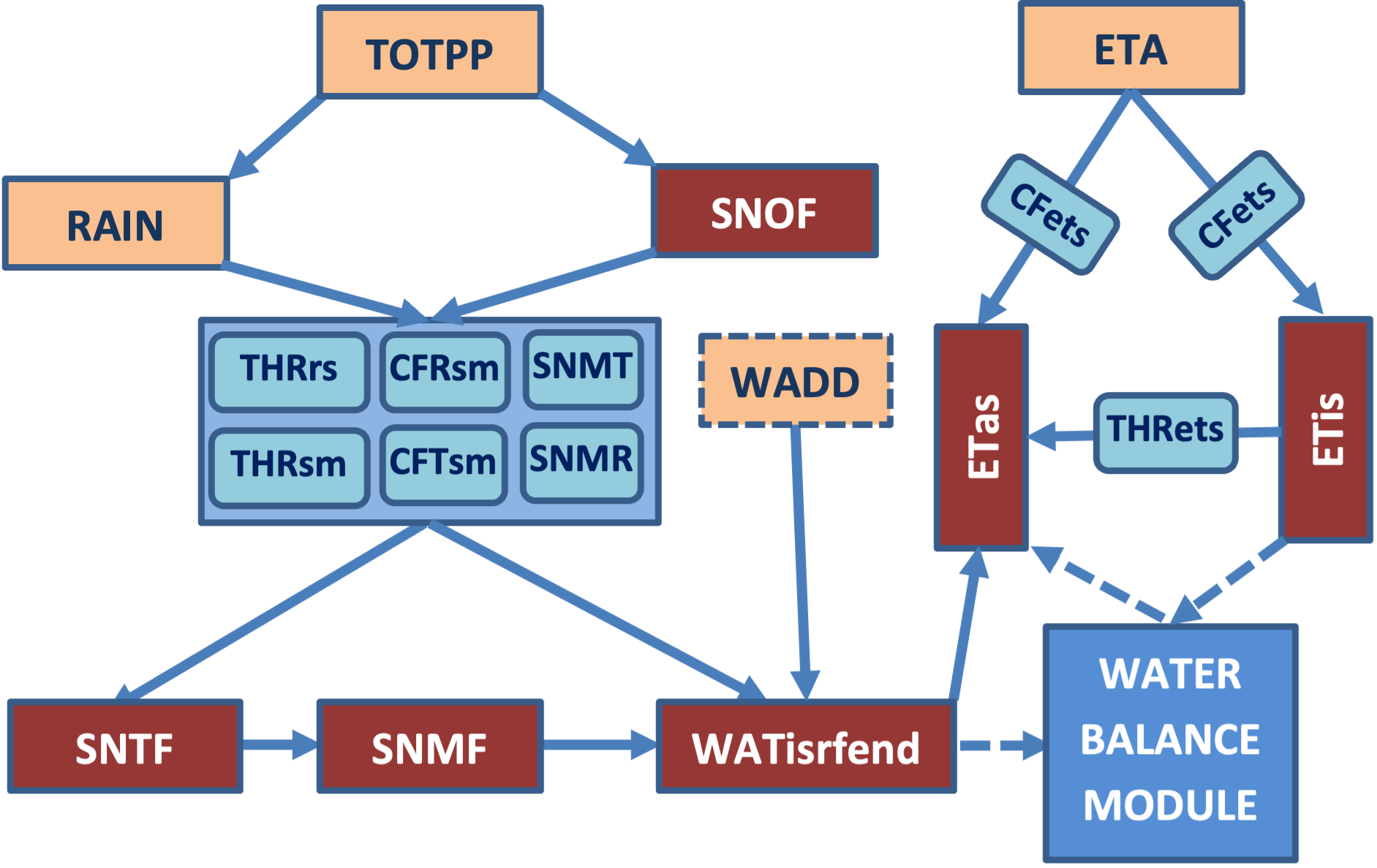
Fig 2. Simplified workflow diagram for the SNOW module
TOTPP - daily total precipitation (input data); RAIN - daily rain (input data); ETA - daily actual (or crop) evapotranspiration (input data); SNOF - Snowfall amount; WADD - water additions from the input file (optional); SNTF - Snow layer thickness; SNMF - (net) snowmelt; WATisrfend - Water available for infiltration or surface runoff; THRrs - Air temperature threshold for rain to be accumulated as snow; THRsm - Air temperature threshold for initiating snowmelt; CFRsm - Correction factor (snowmelt due to rain); CFTsm - Correction factor (snowmelt due to air temperature); SNMT - Snowmelt due to temperature; SNMR - Snowmelt due to rain; Etas - above soil ET; Etis - Soil ET; CFets - Correction factor (portion of evapotranspiration occurring in the soil); THRets - Soil water content threshold for stopping soil evapotranspiration when the soil is dry. Dashed lines indicate output parameters transferred to or from the WATER Balance module.
The input parameters as well as the parameters calculated in the SNOW module are listed in the table below. The parameters in bold are considered to be key output parameters and are the parameters that are shown by default in Table View, while most of the other parameters are shown only if selected by user.
NAME LONG NAME DEFINITION DATE Day (yyyy-mm-dd) Date for analyzed data (required input data). TEMP Temperature (° C) Mean air temperature (required input data). TOTPP Total precipitation (mm) Total precipitation amount (required input data). RAIN Rain (mm) Rain amount (required input data). ETA Evapotranspiration (ET) (mm) Actual evapotranspiration (required input data). WADD Water additions (mm) The amount of water added to the soil from sources other than precipitation (e.g. irrigation, flooding, etc.) (optional input data). The values are zero if the user data is not present or if the user choses not to use the data available in the input file. SNOF Snowfall amount (mm) Snowfall amount (difference between TOTPP and RAIN). RAINS Rain added to the snow layer (mm) Amount of rain that is converted to snow (dependent on THRrs). RAINNS Rain not added to the snow layer (mm) Amount of rain that is preserved as rain (dependent on THRrs). SNOA Snowfall added to the snow layer (mm) Amount of snowfall that is added to the snow layer (dependent on THRsm). SNOM Snowfall not added to the snow layer (mm) Amount of snowfall that is converted to rain. RSSL Rain and snowfall contributing to snow layer (mm) Amount of water from rain and snowfall that is converted to snow and accumulates to the snow layer before temperature and precipitation corrections for the snow layer are applied. RSI Rain and snowfall contributing to infiltration (mm) Amount of water from rain and snowfall that is preserved in liquid form and contributes to water available for infiltration. SNMT Potential snowmelt due to temperature (mm) The amount of snowmelt is dependent on the air temperature. SNMT is calculated using the degree-day concept and is dependent on THRsm and CFTsm. SNMT is used in calculation of SNTFmm and thus, water rerouted to SNMT does not accumulate in the snow layer. SNMR Potential snowmelt due to rain (mm) Rain that is not converted to snow can produce snowmelt. SNMR represents the amount of snowmelt associated with rain. SNMR is calculated as the product of rainfall amount and CFRsm. SNMR is used in calculation of SNTFmm and thus, water rerouted to SNMR does not accumulate in the snow layer. SNTFmm Snow layer thickness (mm) Snow layer thickness (expressed as mm of water) after temperature and precipitation corrections. SNTF represents the final values of snow layer thickness and is a key output parameter. SNG Net snow gain to the snowpack (mm) Net addition of water to the snow layer. SNG represents the net additions to the snowpack and is available only when the snowpack increases between two consecutive days. SNMF Net snowmelt from the snowpack (mm) Net loss of water from the snow layer. SNMF represents water originating from the snow layer that becomes available for infiltration and/or surface runoff and is available only when the snowpack decreases between consecutive days. The assumption is that all the snow that melts become available for infiltration and/or surface runoff instead of being stored in the snow layer. SNTFcm Snow layer thickness (cm) Snow layer thickness (expressed as cm) after temperature and precipitation corrections. SNTFcm is obtained by converting SNTFmm to cm of snow by using CFSmc. SNTFcm represents the final values of snow layer thickness and is a key output parameter. ETasi Above soil ET (mm) before correction for dry soil (mm) Portion of evapotranspiration that occurs above soil. The assumption is that a portion of evapotranspiration occurs in the soil and the reminder occurs above the soil via processes such as canopy interception and/or water ponding at the soil surface. The magnitude of Etasi is controlled by CFets. ETasi can occur only on days when precipitation occurs or snowpack is present, and hence, ETasi is smaller than the value set via CFets. This is an intermediate result that is adjusted via subsequent calculations. ETfsas ET from soil transferred to ET above soil when soil is dry (mm) Evapotranspiration from soil ceases under dry soil conditions (controlled by THRets). THRets allows for transferring ET from soil to ET above ground ET (ETAs) if evaporative demand is still present (ETA) when the soil is dry. The full calculations for ETfsas are performed in the SOIL WATER module. If the SOIL WATER module has not been run, ETfsas is assumed to be zero. Generally, ETfsas is small and hence this limitation is not expected to impact calculations significantly. ETfsas values are adjusted once the SOIL WATER module calculations are performed. ETfsas is the amount transferred from soil ET to above soil ET. ETasf Above soil ET after rerouting ET from dry soil (mm) Portion of evapotranspiration that occurs above soil. The assumption is that a portion of evapotranspiration occurs in the soil and the reminder occurs above the soil via processes such as canopy interception and/or water ponding at the soil surface. The magnitude of Etasf (and ETasi) is controlled by CFets. This is the final result representing the portion of evapotranspiration that occurs above soil and includes corrections for dry soil conditions (ETfsas). WATisrf Water available for infiltration or surface runoff after ET correction (mm) The water amount that is available for either infiltration or surface runoff after ET corrections. WATisrfend Water available for infiltration or surface runoff after all corrections (mm) The water amount that is available for either infiltration or surface runoff after water additions (WADD) are considered. WATisrfend is a key parameter calculated in the SNOW module and is the starting point for the calculations conducted in the WATER BALANCE module. UCD User-provided calibration data If provided, UCD data allows for pairing of SNOSWAB output with data from other sources during the calibration of the model.
3.5. Water Balance Module
The WATER BALANCE module allows for daily estimation of soil water content and of a series of water budget components (e.g., infiltration, drainage, surface runoff). No additional required input time series are needed for this module as all the calculations are based on the output from the SNOW module. For this module the user needs to provide values for several coefficients and adjust settings for the water subtractions routines. The coefficients from this module are used for describing soil properties and for controlling infiltration, drainage, and surface runoff routines. This module also offers the option for setting up thresholds for dry and wet soil state, which can be used for studying soil or crop water deficiency and/or excess. In addition, this module allows for visualization of the water budget and model error using a dynamic water budget diagram and its associated (simplified) table. For a more in-depth evaluation of water deficit and/or excess, together with testing of irrigation scenarios and impacts on aquifer storage the users are encouraged to use SWIB (Soil Water Stress, Irrigation Requirement and Water Balance), another tool included in HTS, and available at https://swib.hydrotools.tech. SWIB requires daily time series of soil water content (SWC), which can be estimated using SNOSWAB or obtained from other sources (e.g., databases of soil moisture measurements, other models, etc.).
Similar to the SNOW module, the user can include one or more calibration time series (e.g., soil water content, groundwater recharge, stream baseflow, surface runoff) in the input file if calibration is to be conducted. Although based on different underlying assumptions, SepHydro hydrograph separation tool available in HTS (https://sephydro.hydrotools.tech) can be used for estimating surface runoff and groundwater discharge components of streamflow, which can be used for example for guiding the calibration of the calculations integrated in the WATER BALANCE module (e.g., surface runoff, drainage).
All the calculations for this module are performed using millimeters of water (mm) units. SWC in model output is available both as mm or as percentage (%). SWC units are converted from millimeters to % and vice versa using the thickness of the soil specified by the user.
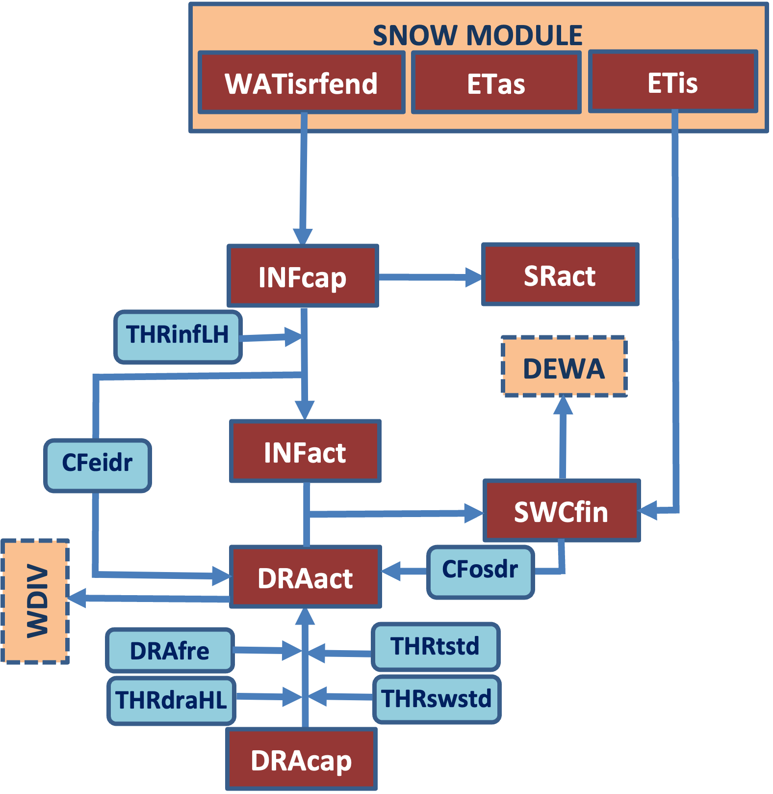
Fig 3. Simplified workflow diagram for the WATER BALANCE module
WATisrfend - Water available for infiltration or surface runoff; Etas - Above soil ET; Etis - Soil ET; INFcap - Infiltration capacity; SRact - Total surface runoff after removing drainage boost; THRinfLH - Soil water content threshold for switching between low and high infiltration rate; DEWA - water subtractions via dewatering (optional); CFeidr - Surface runoff to drainage correction factor (from excess infiltration); INFact - Actual infiltration; SWCfin - Soil water content; WDIV - water subtractions via diversions (optional); DRAact - Actual drainage; CFosdr - Surface runoff to drainage correction factor (from soil oversaturation); DRAfre - Drainage with frozen soil conditions; THRtstd - Air temperature threshold for stopping drainage; THRdraHL - Soil water content threshold for switching drainage from high to low rate (%); THRswstd - Soil water content threshold for stopping drainage; DRAcap - Drainage capacity.
The input parameters as well as the parameters calculated in the WATER BALANCE module are listed in the table below. The parameters in bold are considered to be key output parameters and are the parameters that are shown by default in Table View.
NAME LONG NAME DEFINITION DATE Day (yyyy-mm-dd) Date for analyzed data (required input data). TEMP Temperature (° C) Mean air temperature (required input data). TOTPP Total precipitation (mm) Total precipitation amount (required input data). RAIN Rain (mm) Rain amount (required input data). SNOF Snowfall amount (mm) Snowfall amount (difference between TOTPP and RAIN). ETA Evapotranspiration (ET) (mm) Actual evapotranspiration (required input data). WADD Water additions (mm) [imported from the SNOW module] The amount of water added to the soil from sources other than precipitation (e.g. irrigation, flooding, etc.) (optional input data). The values are zero if the users data is not present or if the user choses not to use the data available in the input file. WDIVinp Water subtractions (diversions) from input file (mm) The amount of water passively removed from the soil layer (e.g. tile drainage). Water Subtractions (Diversions) is subtracted from drainage (DRAact), and is limited by the amount of water available for drainage. Leave the box unchecked if Water Subtractions (Diversions) data is not available in the input file or if the intent is not to use it in calculations. If used, WDIVinp is added to Simulated Water Subtractions (Diversions) (WDIVsim) for calculating the total Water Subtraction (Diversions) (WDIVfin). WDIVsim Simulated water subtractions (diversions) (mm) A fixed portion of the drainage [DRAact] that is removed. The percentage of water diverted from drainage is set using Diversion Efficiency Coefficient (WDIVrat). Leave the box unchecked if the intent is not to simulate water subtraction (diversions). If used, WDIVsim is added to Water Subtractions (Diversions) (WDIVinp) for calculating the total Water Subtraction (Diversions) (WDIVfin). DEWAinp Water subtractions (dewatering) from input file (mm) The amount of amount of water actively removed from the system (e.g. pumping). Water Subtractions (Dewatering) is subtracted from Soil Water Content (SWCdew) and is subject to additional conditions controlling the availability of water for dewatering . Leave the box unchecked if Water Subtractions (Dewatering) data is not available in the input file or if the intent is not to use it in calculations. If used, DEWAinp is added to Simulated Water Subtractions (Dewatering) for calculating the total Water Subtraction (Dewatering) (DEWAf). DEWAsim Simulated water subtractions (dewatering) (mm) A fixed amount of water that is removed from soil water content (SWCdew) and is subject to additional conditions controlling the availability of water for dewatering. The amount of water removed from SWCdew is set using the Dewatering Rate (THRrat), provided SWCdew is above the threshold required for allowing the simulation of dewatering (THRdewsta). Leave the box unchecked if the intent is not to simulate water subtraction (diversions). If used, DEWAsim is added to Simulated Water Subtractions (Dewatering) for calculating the total Water Subtraction (Dewatering) (DEWAf). DEWAsim is currently integrated in DEWAi (and DEWAf) and is not available as a separate output. WATisrfend Water available for infiltration or surface runoff after all corrections (mm) [imported from the SNOW module] The water amount that is available for either infiltration or surface runoff after water additions (WADD) are considered. WATisrfend is a key parameter calculated in the SNOW module and is the starting point for the calculations conducted in the WATER BALANCE module. INFcap Infiltration capacity (mm) Maximum allowed daily infiltration. INFcap is based on either INFlr (low infiltration rate) or INFhr (high infiltration rate) as triggered by THRinfLH. Excess water is transferred to surface runoff when WATisrf > INFcap. INFint Actual infiltration - before surface runoff to drainage correction (mm) Actual infiltration as constrained by WATisrf and INFcap. WATisrf that is in excess of INFcap is re-routed to surface runoff. This is an intermediate result that is adjusted via subsequent calculations. INFact Actual infiltration - after surface runoff to drainage correction (mm) Actual infiltration as constrained by INFint, CFeidr and CFosdr. INFact incorporates all adjustments relative to the infiltration process and is considered a key output parameter. DRAcap Drainage capacity (mm) Maximum allowed daily drainage. DRAcap is based on either DRAlr (low infiltration rate) or DRAhr (high infiltration rate) as triggered by THRdraLH. DRAfre Drainage with frozen soil conditions (mm) DRAcap corrected for frozen soil conditions as triggered by THRtstd. Drainage stops when soil temperature is lower than THRtstd. DRAfin Drainage with dry soil correction (mm) DRAfre corrected for dry soil conditions as triggered by THRswstd. Drainage stops when SWC is lower than THRtstd. DRAfin represents the drainage before surface runoff correction (if any) is applied. DRAbinf Drainage boost from excess infiltration (mm) Excess water is transferred to surface runoff when WATisrf > INFcap. For these cases, drainage can be set to receive a portion of the water directly from surface runoff, as triggered by CFeidr. DRAoss Drainage boost from oversaturated soil (mm) When soil becomes oversaturated, excess water is transferred to surface runoff. For these cases, drainage can be set to receive a portion of the water directly from surface runoff, as triggered by CFosdr. Use of non-zero CFosdr forces the model to bypass SWC calculation. Hence, CFosdr starting values should be zero, and should be adjusted only if model calibration using other coefficients is not satisfactory. DRAact Actual drainage (mm) Actual drainage. DRAact incorporates all adjustments relative to the drainage processes and is considered a key output parameter. WDIVinpcorr Water subtractions (diversions) from input file (mm) after corrections WDIVinp corrected for negative values. WDIVfin Total water subtractions via diversions (mm) The sum of WDIVinp and WDIVsim. This is the portion of drainage (DRAact) that does not become percolation (DEEPP). DEEPP Deep percolation (mm) This is the portion of drainage (DRAact) that is not removed via drainage diversions (WDIVfin) and percolates below the soil layer. ETisi Soil ET (mm) before correction for dry soil Portion of evapotranspiration that occurs in the soil. The assumption is that a portion of evapotranspiration occurs in the soil and the reminder occurs above the soil via processes such as canopy interception and/or water ponding at the soil surface. The magnitude of ETisi is controlled by CFets. This is an intermediate result that is adjusted via subsequent calculations. ETcds Soil ET corrected for dry soil (mm) Evapotranspiration from soil ceases under dry soil conditions (controlled by THRets). ETcds is a key output parameter and is equal to ETisi when the soil is not under dry conditions and zero on the days with dry soil conditions. ETfsas ET from soil transferred to ET above soil when soil is dry (mm) Evapotranspiration from soil ceases under dry soil conditions (controlled by THRets). THRets allows for transferring ET from soil to ET above ground ET (ETAs) if evaporative demand is still present (ETA) when the soil is dry. ETfsas is the amount transferred from soil ET to above soil ET. DEWAi Dewatering before corrections (mm) - intermediate The amount of dewatering not constrained by the soil water content (SWCdew). DEWAf Dewatering after corrections (mm) The amount of dewatering constrained by the availability of water in the soil layer (SWCdew). SWCdew Soil water content (mm) - intermediate SWC (soil water content) after integrating infiltration, drainage, evapotranspiration and dewatering processes. This is an intermediate result as SWC is adjusted via subsequent calculations. SWCfinmm Soil water content - corrected for saturated soil (mm) SWC (soil water content) after SWCint is corrected for saturated soil conditions as set by PORe. SWCfinmm incorporates all adjustments relative to the SWC and is a key output parameter. SWCfin Soil water content - corrected for saturated soil (%) SWC (soil water content) after SWCint is corrected for saturated soil conditions as set by PORe. SWCfin incorporates all adjustments relative to the SWC and is a key output parameter. SReinf Surface runoff due to excess infiltration (mm) Surface runoff due to excess water available for infiltration. Excess water is transferred to surface runoff when WATisrf > INFcap. SReinfDB Surface runoff due to excess infiltration after drainage correction (mm) Surface runoff due to excess water available for infiltration (WATisrf > INFcap) after a portion (controlled by CFeidr) has been re-routed to drainage (DRAbinf). SResas Surface runoff due to saturated soil (mm) Surface runoff due to soil oversaturation (SWC > PORe). When soil becomes oversaturated, excess water is transferred to surface runoff. SResasDB Surface runoff due to saturated soil after drainage correction (mm) Surface runoff due to soil oversaturation (SWC > PORe) after a portion (controlled by CFosdr) has been re-routed to drainage (DRAoss). SRTint Total surface runoff before drainage correction (mm) Total surface runoff, including all adjustments except for drainage correction (DRAbinf and DRAoss). This is an intermediate result that is adjusted via subsequent calculations. SRTact Total surface runoff after drainage correction (mm) SRTact is SRTint after drainage correction (DRAbinf and DRAoss). SRTact incorporates all adjustments relative to the surface runoff processes and is considered a key output parameter. SWCgain Net SWC gain (mm) Soil layer gains water when SWCfinmm on day i+1 is higher than on day i. SWCgain similar to SWCloss over the long-term indicates that the soil water storage is in equilibrium. SWCloss Net SWC loss (mm) Soil layer losses water when SWCfinmm on day i+1 is lower than on day i. SWCloss similar to SWCgain over the long-term indicates that the soil water storage is in equilibrium. SWClow Days with low soil water content Count for days in low SWC state (triggered by THRlw). This is used only for counting the number of days when the soil is in this SWC state and can be used for example for estimating the number of days that require irrigation or number of days with water deficit. SWChigh Days with high soil water content Count for days in high SWC state (triggered by THRlw). This is used only for counting the number of days when the soil is in this SWC state and can be used for example for estimating the number of days with excess water present in the soil. UCD User-provided calibration data If provided, UCD data allows for pairing of SNOSWAB output with data from other sources during the calibration of the model (e.g., soil water content, groundwater recharge, stream baseflow, surface runoff, etc.). -
-
4. User Guide
SNOSWAB (Snow, Soil Water and Water Balance Model) is an online model for obtaining daily estimates of snow related processes (e.g., snowfall, snowmelt, snow layer thickness), soil water content and a series of soil water budget components (e.g., infiltration, drainage, surface runoff) based on user provided daily meteorological (i.e., mean air temperature, total precipitation, rainfall), evapotranspiration and calibration data. The model provides tabular and graphical representations of the input data, output data, and user calibration data (UCD), as well as representative statistics for various time intervals including daily, monthly, meteorological and growing seasons, yearly and various averaging intervals for multiyear data sets (see section 3.2. Time steps and averaging). Calibration routines for each calculation module (i.e., Snow Module, Water Balance Module) are available, and can be used if user calibration data (i.e., UCD) is provided.
At the top, a contextual menu provides access to the various modules available. The modules can be accessed progressively, in the following order: 1) Home (Information module); 2) Input Data (Data entry module); 3) Snow (Calculation module); and 4) Water Balance (Calculation module). Once the calculations of a module are completed, the user can advance to the next module and can also return to the respective module at any time during the session. Additional menu tabs are available for both the data entry (i.e., Info, Load Data, Graphical View, Table View and Export Input Data for the Input Data module) and calculation (i.e., Info, Analysis, Graphical View, Table View and Export Data available for the SNOW and WATER BALANCE modules) modules. In the following sections the options available under the Input Data - Load menu tab and under the Analysis menu tab of each calculation module are presented in separate subsections. The options available under the other menu tabs are common to all three modules mentioned above and are presented as an additional subsection
4.1. Quick start
In order to run SNOSWAB the user has to complete the following steps:
-
Load Data: provide required data or use the provided test data [Input Data module];
-
Perform SNOW calculations: enter required settings and coefficients and select Run Snow Analysis [SNOW module - Analysis]. The calibration of the model is conducted by adjusting the coefficients available on this page in conjunction with the information displayed in the Calibration overlay window, which is launched by using the Run Snow Analysis button;
-
Perform WATER BALANCE module calculations: enter required settings and coefficients and select Run Water Balance Analysis [Water Balance - Analysis]. The calibration of the model is conducted by adjusting the coefficients available on this page in conjunction with the information displayed in the Calibration overlay window, which is launched by using the Run Water Analysis button;
-
Investigate Results and Export Data: review SNOSWAB output from each module [Table View and/or Graphical View] and export results [Export Data button available under each data entry and calculation modules or the CSV button available under the Stats and Calibration Stats of the Graphical View or under the Table, Stats and Calibration Stats of the Table View].
The steps required for using this model are described in more detail below.
4.2. Home Module
This module contains information related to the development, methodology and use of SNOSWAB. Under each of the input and calculation modules an Info tab is available, where general information relevant to the respective module is provided.
4.3. Load Data (Input Data Module)
The first step in conducting an analysis is to upload the input data file to be used in SNOSWAB. The users can run SNOSWAB either by using the test dataset or by uploading a new dataset.
For testing SNOSWAB and better understanding how the various components of the model operate, the user can upload the test data set provided by clicking on "Try the tool using the test dataset” button. The test dataset contains three years of weather input data (required), optional input data and user calibration data (UCD). The optional input time series includes constructed data for simulating water additions (e.g. irrigation, flooding) to and water subtractions (e.g. tile drainage, pumping) from the soil layer, with the users having the option to simulate some of these processes in the absence of water additions and water subtractions data in the input file. UCD data consists of snow layer thickness (cm; UCD1; corresponding to SNOSWAB SNTFcm output parameter; UCD1 measured at Environment and Climate Change Canada [ECCC] Charlottetown weather station, Prince Edward Island, Canada), soil water content (%; UCD2; corresponding to SNOSWAB SWCfin output parameter; UCD2 measured at Agriculture and Agri-Food Canada [AAFC] Harrington Experimental Farm, Prince Edward Island, Canada), surface runoff (mm; UCD3; corresponding to SNOSWAB SRTact output parameter; UCD3 estimated from hydrograph separation of Bell's Creek stream discharge measured at ECCC hydrometric stations in Prince Edward Island, Canada) and stream baseflow (mm; UCD4; corresponding to SNOSWAB DRAact output parameter; UCD4 estimated from hydrograph separation of Bell's Creek stream discharge measured at ECCC hydrometric stations in Prince Edward Island, Canada). Of note, the surface runoff and stream baseflow obtained from hydrograph separation are governed by watershed scale processes, whereas surface runoff and drainage obtained with SNOSWAB are the result of field scale processes. Hence, the calibration of SRTact and DRAact using the data from the test data file (i.e. UCD3 - surface runoff and UCD4 - stream baseflow) is limited.
For using SNOSWAB the users need to upload daily timeseries. The model accepts source data sets in Comma Separated File (csv) format. The users can use the “Download Sample File” button located on the Upload User Data Page (Load Data) or the "Export Input Data - Daily" menu to obtain a correctly formatted input file that can be used as a model for populating the input data file with user data. The “Export Input Data - Daily” menu becomes available after the test or a user dataset is loaded. The user input file can be uploaded to SNOSWAB by using the "Upload user data" button. SNOSWAB allows uploading of files with maximum 7500 rows (~20 years of daily data). It is recommended to split the input data set in blocks of 20 years daily timeseries when the intent is to analyze longer time periods. It should be noted that the model cannot accommodate missing data (i.e., blank rows in required data columns) or erroneous data entries, and hence it is recommended that the integrity of the source data is verified before uploading. An error message will be displayed, and the user will be redirected to the Load Data page if inconsistencies are detected in the user file.
The input data file consists of a tabular file, with the first row dedicated to the parameter names, 1 column dedicated to calendar date, 4 columns dedicated to required input data (TEMP - daily mean air temperature; TOTPP - daily total precipitation; RAIN - daily rain; ETA - daily actual (or crop) evapotranspiration), 3 columns dedicated to optional input data (WADD, WDIVinp, DEWAinp) and 5 columns reserved for optional user calibration data (UCD1 to UCD5). The required input data columns have to contain values in all rows, while the optional data columns can be left blank if data is not available. UCD data sets are not restricted to certain parameters and can include time series for any parameter that the user intends to use for comparing with the output from SNOSWAB. Examples of calibration time series datasets include thickness of snow layer, soil water content, groundwater recharge, stream baseflow, surface runoff, etc.
The number of columns, data format and the units of the various weather parameters required for the input file are shown in the table below.
Columns DATE TEMP TOTPP RAIN ETA WADD WDIVinp DEWAinp UCD (max. 5 cols.) Units yyyy-mm-dd °C mm mm mm mm mm mm user choice Values eg. 2021-12-24 -90 to 60 0 to 1800 0 to 1800 0 to 100 >= 0 >= 0 >= 0 user choice
Notes:
-
Required data:
DATE - use yyyy-mm-dd format;
TEMP - daily mean air temperature;
TOTPP - daily total precipitation;
RAIN - daily rain;
ETA - daily actual (or crop) evapotranspiration; -
Optional data: (leave blank if no data is available)
WADD - daily water additions
WDIVinp - daily water subtractions via diversions
DEWAinp - daily water subtractions via dewatering
UCD - user calibration data (up to five columns) -
The model requires daily data
-
The user input data file has to be uploaded using a file with one column dedicated to calendar date, four columns dedicated to required input data (TEMP, TOTPP, RAIN, ETA), three columns dedicated to optional input data (WADD, WDIVinp, DEWAinp) and up to five columns dedicated to calibration data (UCD1 to UCD5)
-
Use the first row of the data set for column headings
-
SNOSWAB includes limited input data quality check routines and hence, the user must ensure that the input data set is suitable for analysis (e.g., check dataset for missing or erroneous values, etc.)
In the Input Data module the user can specify the beginning and the end of the growing season in the boxes provided. These dates are used for averaging the various parameters during the growing season (GS) and outside of the growing season (OGS) in addition to other averaging periods. In SNOSWAB, it is assumed that these dates are not changing from year to year and hence, the start and end dates use the mm-dd format (the year is ignored as the same dates are applied to all years available in the input data file).
Once the input dataset is loaded to SNOSWAB via either the "Try the tool using the test data set" or "Upload user data" button an overlay window appears (i.e., "Select the UCD averaging method") asking the user to specify the method used for calculation of monthly values for each UCD timeseries (i.e., averaging vs. summation). Once this step is completed a new button ("UCD") is added to the right of the Input Data tab at the top of the page and the view switches to Graphical View. The UCD menu available at the top of the page allows the user to change the method for the calculation of monthly values for each UCD at any time. See section 4.7. for instructions regarding the inspection of datasets using tables and graphs as well as for the various options available for exporting the data.
Once the loading and inspecting of the input data is completed the user can click on the SNOW menu entry at the top of the page to advance to the first calculation module.
Consult section 3.1. and section 3.3. for more details.
4.4. Analysis - Snow Module
On the Analysis Tab the user can adjust model run settings and provide a series of coefficients according to the list of coefficients and instructions provided in the table included in section 3.3. - SNOW Module (Model Coefficients).
Once the settings for the Water Additions routine and values for the Starting values and Coefficients are set and the user selects the pairs of datasets to be used during the calibration (i.e., Calibration mapping menu), the user can click on the Run Snow Analysis button and the Calibration overlay window will be displayed. The amount of water available for infiltration (WATisrf) calculated with this module, might be impacted by the calculations performed for the WATER BALANCE module for the periods when soil moisture is lower than the threshold for stopping evapotranspiration from soil when the soil is dry (i.e., THRets). The respective calculations have minimal impact (or no impact) on the snowpack processes (e.g., melting, accumulation, etc.) as the dry soil condition for stopping evapotranspiration from soil is typically triggered during the warmer periods of the year (i.e., summer), when the snowpack is not present. See section 4.5. for more details regarding how the calculation from WATER BALANCE module impact the calculations in the SNOW module. The model settings, the Starting values and the Coefficients can be subsequently adjusted during the calibration procedure, with calibration being considered final once no further improvement in the model fitness is observed. Upon completion of the calibration procedure the view switches to Graphical View. For this module, an additional tab (i.e.; “Water Budget”) includes a dynamic water budget diagram (accessible via the “Diagram” tab) and a water budget (simplified) table (accessible via the “Table” tab).
See section 4.6. for instructions regarding the calibration of the model and section 4.7. for instructions regarding the inspection of datasets using tables and graphs as well as for the various options available for exporting the data.
The user can click on the Water Balance menu entry at the top of the page to advance to the next calculation module.
Consult section 3.3. and section 3.4. for more details.
4.5. Analysis - Water Balance Module
On the Analysis Tab the user can adjust model run settings and provide a series of coefficients according to the list of coefficients and instructions provided in the table below included in section 3.3. - WATER BALANCE Module (Model Coefficients).
Once the settings for the Water Subtractions routines (either as diversions or dewatering) and values for the Starting values and Coefficients are set and the user selects the pairs of datasets to be used during the calibration (i.e., Calibration mapping menu), coefficient values are set the user can click on the Run Snow Analysis button and the Calibration overlay window will be displayed. Of note, calculations in this module account for a threshold for stopping evapotranspiration from soil when the soil is dry (i.e., THRets). When the soil moisture is lower than this threshold, all evapotranspiration is considered to occur before the water enters the soil, thus overriding the correction factor for the portion of evapotranspiration occurring in soil (i.e., CFets). When this condition is triggered, the calculation of the amount of water available for infiltration (WATisrf), calculated in the SNOW module (and carried over into the Water Balance Module) is impacted. Thus, when WATER BALANCE calculations are conducted, they also result in recalculation of the SNOW module. Importantly, the recalculations have minimal impact (or no impact) on the snowpack processes (e.g., melting, accumulation, etc.) as the dry soil condition for stopping evapotranspiration from soil is typically triggered during the warmer periods of the year (i.e., summer), when the snowpack is not present. The model settings, the Starting values and the Coefficients can be subsequently adjusted during the calibration procedure, with calibration being considered final once no further improvement in the model fitness is observed. Upon completion of the calibration procedure the view switches to Graphical View. For this module, an additional tab (i.e.; “Water Budget”) includes a dynamic water budget diagram (accessible via the “Diagram” tab) and a water budget (simplified) table (accessible via the “Table” tab).
See section 4.6. for instructions regarding the calibration of the model and section 4.7. for instructions regarding the inspection of datasets using tables and graphs as well as for the various options available for exporting the data.
Consult section 3.3. and section 3.5. for more details.
4.6. Model Calibration
Calibration of the model is performed via the Analysis tab of each of the calculation modules (i.e., SNOW and WATER BALANCE). Calibration is conducted by first pairing the output of the model with the user calibration data (UCD) using the “Calibration mapping” menu available under the “Analysis” tab of each calculation module. For example, SNTFcm [Snow layer thickness, mm] in SNOW module output can be paired with measured snow thickness if available. Once the pairing is completed, the user can proceed to running the respective module (i.e., “Run Snow Analysis” or “Run Water Balance Analysis” button at the bottom of the Analysis tab page) and inspect the fitness of the model in the subsequent Calibration overlay window. The fitness of the model for various timesteps and averaging intervals can be inspected in the Calibration overlay window via graphs as well as bivariate statistics. In addition, the “Water Budget” tab (available in the “Water Balance module” once a model run has been completed) includes calculations of the model error, which can be visualized using either the dynamic water budget diagram or its associated (simplified) table. If the calibration is considered unsatisfactory the user can return to the Analysis menu (i.e., "Return" button), adjust the various coefficients of the model and rerun the analysis. If the calibration is considered satisfactory the user can complete the calculations by proceeding to the next step (i.e., "Proceed to results" in the Calibration Overlay window).
To aid with data inspection and assessment of the fitness of the model SNOSWAB includes several univariate and bivariate statistics. Univariate statistics, including average, minimum, maximum and standard deviation are calculated separately for the input (i.e., user provided calibration data) and model output time series. The graphs and the univariate statistics can be used for example for comparing the general trends, the range of values and the amplitude of variations in both data sets. The bivariate statistics include the coefficient of determination (R2), root mean square error (RMSE), the normalized root mean square error (NRMSE) and the percentage bias (PBIAS). NRMSE is calculated by using the average, the interquartile range or the differences between maximum and minimum (see definitions below). The bivariate statistics are used for evaluating the fitness of the model, by providing a measure of the differences between the values calculated by the model and the user provided calibration data (i.e., UCD). The equations used for calculating each bivariate statistic are shown below.
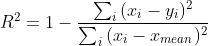
Eq 1. - Coefficient of determination
R2 - coefficient of determination
xi - value for observed data on day i
yi - value for modelled data on day i
xmean - mean of observed data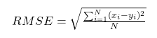
Eq 2. - Root mean square error
RMSE - Root mean square error
N - number non-missing data points
xi - value for observed data on day i
yi - value for modelled data on day i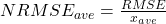
Eq 3. - Normalized root mean square error average
NRMSEave - normalized root mean square error calculated using the average value of measured data
RMSE - root mean square error
xave - average value of observed data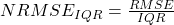
Eq 4. - Normalized root mean square error IQR
NRMSEIQR - normalized root mean square error calculated using minimum and maximum values of measured data
RMSE - root mean square error
IQR - interquartile range of the observed data; IQR = Q3-Q1,
with Q3 = CDF-1(0.25), Q1 = CDF-1(0.75),
where CDF is the quantile function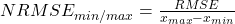
Eq 5. - Normalized root mean square error min/max
NRMSEmin/max - normalized root mean square error calculated using minimum and maximum values of measured data
RMSE - root mean square error
xmax - maximum value for observed data
xmin - minimum value for observed data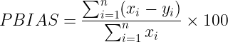
Eq 6. - Percentage Bias
PBIAS - Percentage Bias (%)
xi - value for observed data on day i
yi - value for modelled data on day i
The model error, which is defined as the difference between the water inputs to the soil and the sum of water outputs from the soil, change in soil water storage and change in snow water storage, is generally considered acceptable when it is less than 10%. The model error is calculated both as mm of water and as relative error (i.e.; %) using the following equations:

Eq 7. - Absolute error of the model
Emm - absolute error of the model [mm]
INP - sum of water inputs to the soil [mm]
OUT - sum of water outputs from the soil [mm]
ΔSWC - change in soil water storage (i.e.; difference between storage on the last day and storage for the first day of the analyzed interval) [mm]
ΔSNO - change in snow water storage (i.e.; difference between storage on the last day and storage for the first day of the analyzed interval) [mm]
Eq 8. - Sum of water inputs to the soil
INP - sum of water inputs to the soil [mm]
SNOF - snowfall [mm]
RAIN - rainfall [mm]
WADD - water additions from input file [mm]

Eq 9. - Sum of water outputs from the soil
OUT - sum of water outputs from the soil [mm]
DEWAf - dewatering after corrections [mm]
ETasf - above soil ET [mm]
ETcds - soil ET [mm]
SRTact - total surface runoff [mm]
DEEPP - deep percolation [mm]
WDIVfin - water subtractions via diversions [mm]

Eq 10. - Relative error of the model
E(%) - relative error of the model [%]
OUT - sum of water outputs from the soil [mm]
INP - sum of water inputs to the soil [mm]
It is recommended that the calibration is conducted by changing one coefficient at a time over a selected range of values. When no further improvement is observed in the model output the user can advance to adjusting the values of the next coefficient. The values of the various coefficients can be considered final once no further improvement in the model fitness is observed. Currently, only calibration by trial and error is available, however the integration of an autocalibration routine in SNOSWAB is in planning stages.
4.7. Data inspection, visualisation and export (all modules)
Inspection of data via graphical and tabular views can be conducted via the Graphical View, Table View and Export Data menu entries that become available in the Input Data module once the input dataset is loaded to SNOSWAB. These menu entries are also available under each of the calculation modules (SNOW and WATER BALANCE) and allow the user to evaluate the output for each of these modules.
Graphical View allows for plotting of input or output data using various time steps and intervals (see Section 3.2. Time steps and averaging for more details) available via a drop-down menu. The parameters that can be displayed are available in the selection pane located to the right of the plot. Each parameter can be displayed on the primary (left) Y axis or on the secondary (right) Y axis by clicking on the toggle placed at the right of the selection pane. Additional options for customizing the plot become visible in the top right corner when the mouse pointer is placed above the plot. These options include zoom, auto scale, reset axes, show data point labels, download plot, etc. Univariate statistics (average, minimum, maximum, standard deviation) for selected timeseries and bivariate statistics (R2, RMSE, NRMSEave, NRMSEIQR, NRMSEmin/max, PBIAS) for inspecting the fitness of the model are available under the Stats and Calibration Stats tabs, respectively. These statistics are available either for the entire dataset ("Show Complete Dataset Stats" button) or for a selected subset ("Show stats by Interval" button). The tables shown on the statistics pages can be exported individually by using the corresponding CSV button located to the right of the page. The “Water Balance” module includes under the “Water Budget” tab a dynamic water budget diagram (accessible via the “Diagram” tab) that allows for visualization of key outputs from the calculations conducted in this module for the various averaging periods. The Water Balance diagram can be exported as image either via screen capture of by using the “Export diagram” button available on this page.
Table View allows the user to display data in tabular format using various time steps and intervals (see Section 3.2. Time steps and averaging for more details). The user can also change the number of lines, filter data based on date or adjust the starting date of the data that is displayed. In the initial Table View, the columns displayed are limited to mostly "key" parameters, however the user can change the selection of the parameters to be displayed by selecting the parameters listed above the table. In the respective list, the parameters that are displayed in the table are shown in filled boxes, while the ones that are omitted are included in clear boxes. The “key” parameters are shown in red font. Similar to the Graphical View, univariate statistics (average, minimum, maximum, standard deviation) for selected timeseries and bivariate statistics (R2, RMSE, NRMSEave, NRMSEIQR, NRMSEmin/max, PBIAS) for inspecting the fitness of the model are available under the Stats and Calibration Stats tabs, respectively. These statistics are available either for the entire dataset (“Show Complete Dataset Stats” button) or for a selected subset (“Show stats by Interval” button). The tables shown on the statistics pages can be exported individually by using the corresponding CSV button located to the right of the page. The “Water Balance” module includes under the “Water Budget” tab a simplified water budget table (accessible via the “Table” tab), which includes the key outputs from the calculations conducted in this module. The Water Balance table can be exported by using the “CSV” button available on this page.
The Export Data tab offers additional options for exporting the entire dataset using various time steps and intervals (see Section 3.2. Time steps and averaging for more details). The Export Data tab also provides options for exporting statistics and configuration (i.e., values of parameters and coefficients used by the user in the respective module) The data is currently exported in csv format. The csv button located at the top right of each table in Table View or in Graphical View can be used if the intent is to export only the data shown in the current window.
-
-
5. Limitations
SNOSWAB allows uploading of files with maximum 7500 rows (~20 years of daily data). It is recommended to split the input data set in blocks of 20 years daily timeseries when the intent is to analyze longer time periods.
SNOSWAB includes limited input data quality check routines. Hence, the user is advised to conduct a thorough data quality check before uploading input data to minimize the risk for erroneous output.
-
6. Terms of Use
SNOSWAB can be used freely.
The authors do not assume any responsibility for the model's operation, output, interpretation, or use of results.
-
7. Contact
Serban Danielescu, Ph.D.
Research Scientist | Chercheur scientifique
Environment and Climate Change Canada | Environnement et Changements Climatiques Canada
Agriculture and Agri-Food Canada | Agriculture et Agroalimentaire Canada
Fredericton Research and Development Centre | Centre de recherche et développement de Fredericton
95 Innovation Rd., Fredericton, NB, E3B 4Z7
Telephone/Téléphone: 506-460-4468
Facsimile/Télécopieur: 506-460-4377
